You can create a PE correction curve immediately after acquiring data or use the log file created in a previous session. PEMPro places all log files in the directory specified in the Logs and Images Dir field on the Setup tab of PEMPro's main window.
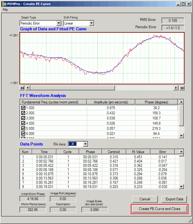
When the create PE Curve dialog opens it may take a few seconds to calculate an optimum curve. In most cases you won't need to do any modifications to the curve. Advanced users may wish to add or remove fundamental frequencies to see how that effects the curve's fit, the measure of which is the RMS Error in the upper right of the dialog.
Before leaving this dialog take a moment to check that the Worm Period, Image Roll, Declination, and Image Scale look correct. If anything looks wrong click Cancel and go back to the Setup and Calibration Wizard to setup the parameters again. Otherwise press Create PE Profile and Close if you are satisfied with the curve. For more details on other features of this page see below.
After the Create PE Curve dialog closes in the previous step, PEMPro will automatically switch to the Program Mount tab and ask if you want to upload to the mount. If you click Yes the curve is immediately uploaded to the mount and you are done! If you want to see more details on the program mount page click here.
Create PEC Curve Dialog
Note: the curve-fitting calculations are CPU intensive and could take seconds or even tens of seconds to calculate the best-fitting Fourier-series. A small pop-up dialog appears and an hour-glass cursor appears while processing so you know calculations are going on. Everything is recalculated if you change RA Axis or change the drift fitting polynomial.
Most of the calculations and fit optimizations are hidden and occur automatically. This dialog is separated into three sections. The top is the graph area which will display the PE curve and data points.
Note that there is a scroll bar below the graph which allows you to scroll across the data to see how it matches the all of the PE data you are analyzing. There are also buttons on the left and right of the scroll bar that allow you to jump exactly one worm period ahead or behind (unless you have reached the beginning or end of the data). Also, as you move the mouse over the graph the current relative time of the data (X-Axis) and the arc-seconds (Y-axis) are displayed above the graph.
Graph Type
There are four graph types: Periodic Error, Error Histogram, Frequency Spectrum, and Frequency Spectrum(secs).
Periodic Error: Shows the fitted curve that PEMPro created against the original data. This is the default display when this dialog opens. Moving the cursor over the graph window will show the phase of the mount (x-axis) and arc-seconds (y-axis).
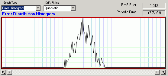
Error Histogram: When selected the graph will show the histogram plot of the errors (last column in the Data Points Table). This histogram plot shows the distribution of these errors. If the distribution is broad then the PE curve is not likely very accurate. If it is asymmetrical that might signal a physical problem.
Moving the mouse over the graph will display the error value and the number of instances found for it. The blue line is the center-point (0 arc-sec error). The buttons to the left and right of the scroll bar on the bottom allow you to increase or decrease the resolution of the histogram.
Moving the cursor over the graph window will show the arc-seconds error (x-axis) and the number of instances in the data where this amount of error occurred (y-axis).
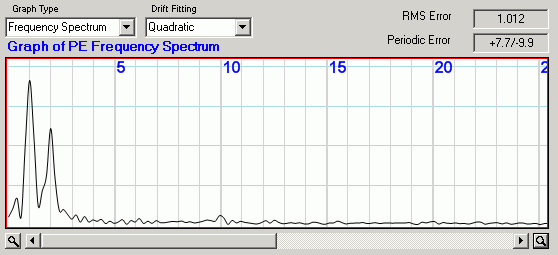
Frequency Spectrum: Shows the periodic error components in inverse units of "worm periods". For example in the picture below there are major humps at 1, 2, and small humps at about 0.5 and 10.
In physical terms this means that this mount, which has a worm period of 382.95 seconds has repeating errors at:
382.95 / 1 = 382.95 seconds (Worm period divided by 1.)
382.95 / 2 = 191.48 seconds (Worm period divided by 2.)
382.95 / 10 = 38.29 seconds (worm period divided by 10
382.95 / 0.5 = 765.9 seconds (this could be real harmonic but is probably just drift fitting error)
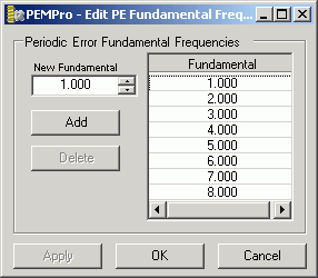
Once you note the fundamentals you can customize PEMPro to look at only those fundamentals with the menu option: File | Edit Fundamentals. which is described below.
Moving the cursor over the graph window will show the frequency in multiples of worm period error (x-axis) and the arc-seconds error (y-axis) of this component. The amplitude of of the data peaks may not match the amplitudes in the FFT Waveform Analysis table because the peaks have a non-zero width and the actual amplitude is related to the area under the peak.
Frequency Spectrum(secs): Shows the periodic error components in units of seconds. Moving the cursor over the graph window will show the frequency in seconds (x-axis) and the arc-seconds error (y-axis) of this component. The amplitude of of the data peaks may not match the amplitudes in the FFT Waveform Analysis table because the peaks have a non-zero width and the actual amplitude is related to the area under the peak.
FFT Waveform Analysis: This table has the fundamental waveforms of the period of the worm gear. PEMPro automatically calculates the optimized values for each fundamental and displays the amplitude and phase.
You can check or uncheck each fundamental to see how the waveform changes. As you do this watch the Total RMS Error in the upper right. This is a measure of “goodness of fit” of the curve to the data. The lower the RMS Error, the better the fit. That shows the root-mean square error in arc-seconds of the fitted PE curve to the data.
Below this is the Periodic Error of your mount in arc-seconds as calculated by the terms in use. Important: be sure that the Image Scale value in the lower left corner is correct for your camera. If it is not you need to Cancel this dialog, change the image scale in the Analyze page and come back to this dialog.
If you are not sure which axis is the RA axis you can switch between axes with the RA Axis combo box.


 Edit Fundamentals: Use this option to edit the fundamentals. This is usually used in conjunction with the Frequency Spectrum graph.